Displaying & Visualisation
Printing/displaying Info
Current info
  state = [0,0,0,1,0]
  fpoly = [5,4,3,2]
  L = LFSR(fpoly=fpoly,initstate =state, verbose=True)
  L.info()


5-bit LFSR with feedback polynomial  x^5 + x^4 + x^3 + x^2 + 1 with
Expected Period (if polynomial is primitive) =  31
Computing configuration is set to Fibonacci with output sequence taken from 5-th (-1) register
Current :
State        :  [0 0 0 1 0]
Count        :  0
Output bit   :  -1
feedback bit :  -1
print(L)

      LFSR ( x^5 + x^4 + x^3 + x^2 + 1)
      ==================================================
      initstate       =       [0 0 0 1 0]
      fpoly           =       [5, 4, 3, 2]
      conf            =       fibonacci
      order           =       5
      expectedPeriod  =       31
      seq_bit_index   =       -1
      count           =       0
      state           =       [0 0 0 1 0]
      outbit          =       -1
      feedbackbit     =       -1
      seq             =       [-1]
      counter_start_zero      =       True
Parameters setting
repr(L)
“LFSR(‘fpoly’=[5, 4, 3, 2], ‘initstate’=[0, 0, 0, 1, 0],’conf’=fibonacci, ‘seq_bit_index’=-1,’verbose’=True, ‘counter_start_zero’=True)”
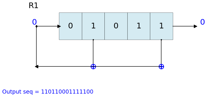
Visualise LFSR
Plotting LFSR with pylsr
Each LFSR can be visualize as it in current state by using .Viz() method
L = LFSR(initstate=[1,1,0,1,1],fpoly=[5,2])
L.runKCycle(15)
L.Viz(title='R1')
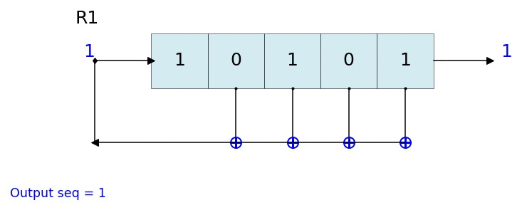
Dynamic visualisation of LFSR - Animation
%matplotlib notebook
L = LFSR(initstate=[1,0,1,0,1],fpoly=[5,4,3,2],counter_start_zero=False)
fig, ax = plt.subplots(figsize=(8,3))
for _ in range(35):
  ax.clear()
  L.Viz(ax=ax, title='R1')
  plt.ylim([-0.1,None])
  #plt.tight_layout()
  L.next()
  fig.canvas.draw()
  plt.pause(0.1)
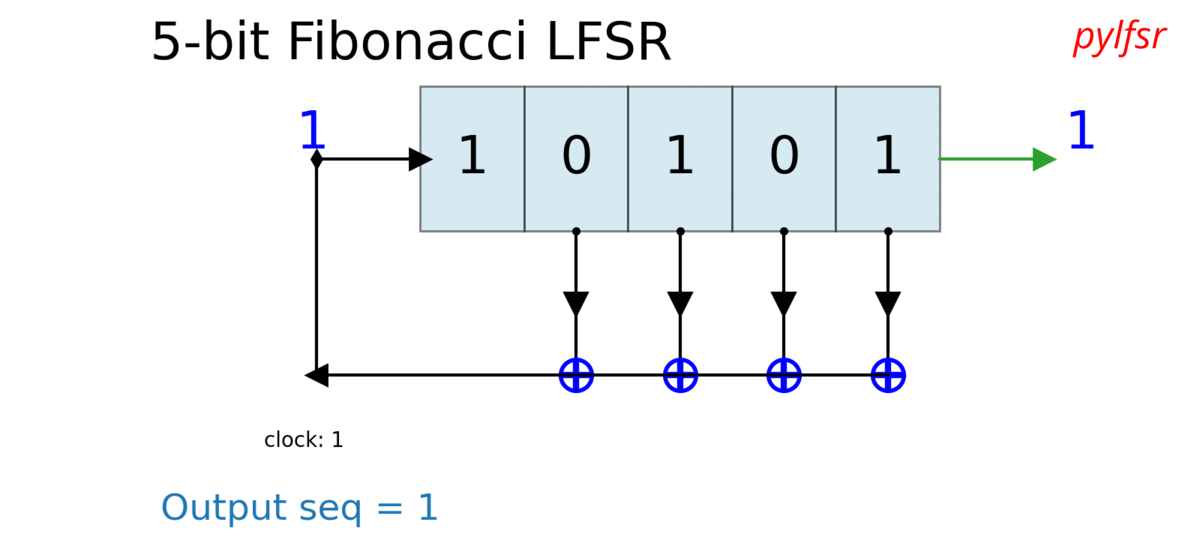
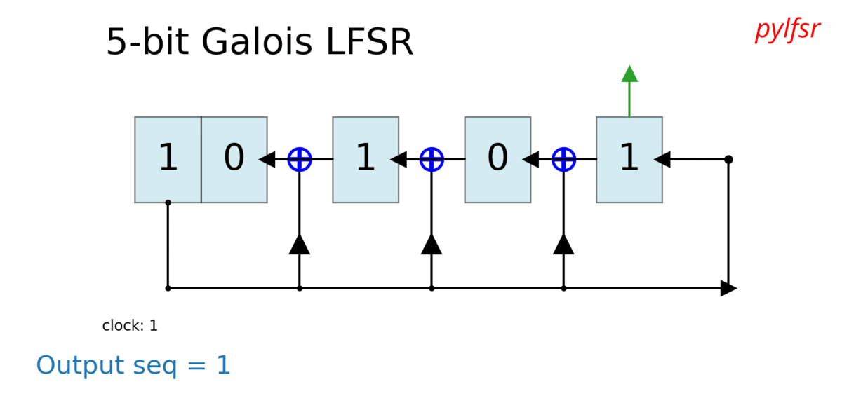
Similarly other can be created as
Show each state and each cycle
Setting clock start:
Initial output bit An argument counter_start_zero can be used to initialize the output bit. * If counter_start_zero=True (default), the output bit is initialize by -1, to illustrate that No clock is provided yet.
In this case, cout (counter) starts with 0. The first output is not computed until first cylce is executed, such as by executing .next(), .runFullCycle, etc
If counter_start_zero=False, the output bit is initialize by the last bit of register. In one sense, first clock cycle is executed. This is why, in this case, cout (counter) starts with 1.
In both cases counter_start_zero =True or False, the L.seq will be same, the only difference is the total number of output bits produced after N-cycles, i.e. when setting counter_start_zero = False, there will be one extra bit, since first bit was already computed. To understand this, look at following two examples. counter_start_zero=True can be seen as dealyed response by one bit.
Visualise 3-bit LFSR
At each step, with default ‘counter_start_zero = True’
state = [1,1,1]
fpoly = [3,2]
L = LFSR(initstate=state,fpoly=fpoly)
print('count \t state \t\toutbit \t seq')
print('-'*50)
for _ in range(15):
    print(L.count,L.state,'',L.outbit,L.seq,sep='\t')
    L.next()
print('-'*50)
print('Output: ',L.seq)
count          state          outbit   seq
--------------------------------------------------
0             [1 1 1]         -1      [-1]
1             [0 1 1]         1       [1]
2             [0 0 1]         1       [1 1]
3             [1 0 0]         1       [1 1 1]
4             [0 1 0]         0       [1 1 1 0]
5             [1 0 1]         0       [1 1 1 0 0]
6             [1 1 0]         1       [1 1 1 0 0 1]
7             [1 1 1]         0       [1 1 1 0 0 1 0]
8             [0 1 1]         1       [1 1 1 0 0 1 0 1]
9             [0 0 1]         1       [1 1 1 0 0 1 0 1 1]
10            [1 0 0]         1       [1 1 1 0 0 1 0 1 1 1]
11            [0 1 0]         0       [1 1 1 0 0 1 0 1 1 1 0]
12            [1 0 1]         0       [1 1 1 0 0 1 0 1 1 1 0 0]
13            [1 1 0]         1       [1 1 1 0 0 1 0 1 1 1 0 0 1]
14            [1 1 1]         0       [1 1 1 0 0 1 0 1 1 1 0 0 1 0]
--------------------------------------------------
Output:  [1 1 1 0 0 1 0 1 1 1 0 0 1 0 1]
At each step, with default ‘counter_start_zero = False’
state = [1,1,1]
fpoly = [3,2]
L = LFSR(initstate=state,fpoly=fpoly,counter_start_zero=False)
print('count \t state \t\toutbit \t seq')
print('-'*50)
for _ in range(15):
    print(L.count,L.state,'',L.outbit,L.seq,sep='\t')
    L.next()
print('-'*50)
print('Output: ',L.seq)
count          state          outbit   seq
--------------------------------------------------
1     [1 1 1]         1       [1]
2     [0 1 1]         1       [1 1]
3     [0 0 1]         1       [1 1 1]
4     [1 0 0]         0       [1 1 1 0]
5     [0 1 0]         0       [1 1 1 0 0]
6     [1 0 1]         1       [1 1 1 0 0 1]
7     [1 1 0]         0       [1 1 1 0 0 1 0]
8     [1 1 1]         1       [1 1 1 0 0 1 0 1]
9     [0 1 1]         1       [1 1 1 0 0 1 0 1 1]
10    [0 0 1]         1       [1 1 1 0 0 1 0 1 1 1]
11    [1 0 0]         0       [1 1 1 0 0 1 0 1 1 1 0]
12    [0 1 0]         0       [1 1 1 0 0 1 0 1 1 1 0 0]
13    [1 0 1]         1       [1 1 1 0 0 1 0 1 1 1 0 0 1]
14    [1 1 0]         0       [1 1 1 0 0 1 0 1 1 1 0 0 1 0]
--------------------------------------------------
Output:  [1 1 1 0 0 1 0 1 1 1 0 0 1 0 1]
