Examples

Construction of LFSR

To create an LFSR, all you need is feedback polynomial p(x) and initial state of LFSR. Feedback polynomial is passed as `fpoly` and initial state is passed as `initstate`

For feebback polynomial p(x) = x⁵+ x⁴+ x³+ x²+1, `fpoly = [5, 4, 3, 2]` Initial state can be passed as string {‘ones’ or ‘random’} or list of binary vector `initstate = [1,0,0,1,1]`

Order of polynomial should be less than equal to register size which is decided by given initial state vector.

While creating LFSR, configuration can also be choosed as str {‘fibonacci’, ‘galois’}, defualt setting is ‘fibonacci’

Output stream by default is taken from last register, however, it can be choosen to any one of registers by setting `seq_bit_index`

Basic Examples

5-bit LFSR with p(x) = x⁵+ x²+1

Default feedback polynomial is p(x) = x⁵+ x²+ 1 and default initial state is all ones

import numpy as np
from pylfsr import LFSR

L = LFSR()

# print the info
L.info()

5 bit LFSR with feedback polynomial  x^5 + x^2 + 1
Expected Period (if polynomial is primitive) =  31
Current :
State        :  [1 1 1 1 1]
Count        :  0
Output bit   : -1
feedback bit : -1

Execute cycle(s)

Run LFSR by clock

To execute one cycle or multiple cycles `next()` or `runKCycle(k)` is used One full period can also be execute by using `runFullPeriod()`

# one cycle
L.next()

# K cycles
k=10
seq  = L.runKCycle(k)

#Cycles of a full period, #cycles = expected period of LFSR

# L.runFullCycle()  # Depreciated

seq = L.runFullPeriod()

5-bit LFSR with p(x) and initial state

To create 5-bit LFSR of feedback polynomial p(x) = x⁵+ x⁴+ x³+ x²+1, and choosen initial state, here is a simple example

state = [0,0,0,1,0]
fpoly = [5,4,3,2]
L = LFSR(fpoly=fpoly,initstate=state, verbose=True)
L.info()

L.Viz()

5-bit LFSR with feedback polynomial  x^5 + x^4 + x^3 + x^2 + 1 with
Expected Period (if polynomial is primitive) =  31
Computing configuration is set to Fibonacci with output sequence taken from 5-th (-1) register
Current :
State        :  [0 0 0 1 0]
Count        :  0
Output bit   :  -1
feedback bit :  -1

Fibonacci LFSR

By deault, LFSR is in Fibonacci configuration mode, but it can be implicitly set to Fibonacci configuration by using `conf`

fpoly = [14, 8, 6, 1]
L = LFSR(fpoly=fpoly,initstate='random', conf='fibonacci')
L.Viz(show_outseq=False)

Galois LFSR

To construct LSFR with Galois configuration , pass `conf = 'galois'`

L = LFSR(fpoly = [5,4,3,2], conf='galois')
L.Viz(show_outseq=False)

23-bit LFSR: x²³+ x¹⁸+1

L = LFSR(fpoly=[23,18],initstate ='random',verbose=True)
L.info()
L.runKCycle(10)
seq = L.seq

23-bit LFSR with feedback polynomial  x^23 + x^18 + 1 with
Expected Period (if polynomial is primitive) =  8388607
Computing configuration is set to Fibonacci with output sequence taken from 23-th (-1) register
Current :
State        :  [0 1 0 1 0 1 0 0 0 1 0 1 0 0 0 1 1 0 1 1 1 0 0]
Count        :  0
Output bit   :  -1
feedback bit :  -1
S:  [0 1 0 1 0 1 0 0 0 1 0 1 0 0 0 1 1 0 1 1 1 0 0]
S:  [0 0 1 0 1 0 1 0 0 0 1 0 1 0 0 0 1 1 0 1 1 1 0]
S:  [1 0 0 1 0 1 0 1 0 0 0 1 0 1 0 0 0 1 1 0 1 1 1]
S:  [0 1 0 0 1 0 1 0 1 0 0 0 1 0 1 0 0 0 1 1 0 1 1]
S:  [1 0 1 0 0 1 0 1 0 1 0 0 0 1 0 1 0 0 0 1 1 0 1]
S:  [1 1 0 1 0 0 1 0 1 0 1 0 0 0 1 0 1 0 0 0 1 1 0]
S:  [0 1 1 0 1 0 0 1 0 1 0 1 0 0 0 1 0 1 0 0 0 1 1]
S:  [0 0 1 1 0 1 0 0 1 0 1 0 1 0 0 0 1 0 1 0 0 0 1]
S:  [1 0 0 1 1 0 1 0 0 1 0 1 0 1 0 0 0 1 0 1 0 0 0]
S:  [1 1 0 0 1 1 0 1 0 0 1 0 1 0 1 0 0 0 1 0 1 0 0]

23-bit LFSR: x²³+ x⁵+1

L = LFSR(fpoly=[23,5],initstate ='ones')
L.info()
#L.runFullPeriod()
L.runKCycle(10000)
seq = L.seq
L.arr2str(seq)

'1111111111111111111111100000111110000011111000110000011
10011111000110111101100111110001101110100110000011100100
01010110011100100101101001111111000111000101011001001100
01011010011111110110001110101001101100110101110110111110
10010010001010100010110001000110011001110110001110010000
01001100101000100011000100010001110010100011001110111110
01100111010111011001000001001100110111011100111011101110
11001101111100100100111111100100110000101000...

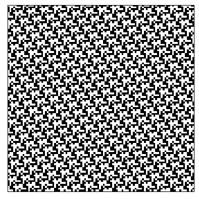
Output as Binary Image

import numpy as np
import matplotlib.pyplot as plt
from pylfsr import LFSR

L = LFSR(fpoly=[23,5],initstate ='ones')
L.runKCycle(10000)
seq = L.seq
I = seq.reshape([100,100])
plt.imshow(I,cmap='gray')
plt.xticks([])
plt.yticks([])
plt.show()

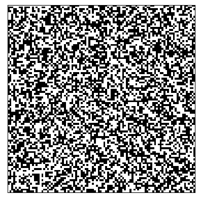
L = LFSR(fpoly=[8, 4, 3, 2],initstate ='ones')
#L.info()
L.runKCycle(10000)
seq = L.seq
I = seq.reshape([100,100])
plt.imshow(I,cmap='gray')
plt.xticks([])
plt.yticks([])
plt.show()

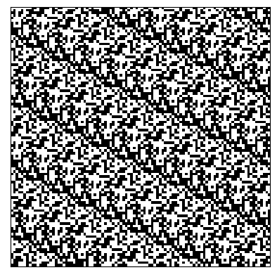
L = LFSR(fpoly=[5,3],initstate ='ones')
#L.info()
L.runKCycle(10000)
seq = L.seq

I = seq.reshape([100,100])
plt.imshow(I,cmap='gray')
plt.xticks([])
plt.yticks([])
plt.show()